3 Amazing Excel Tricks For Marketers For Better Data Analysis

At the risk of sounding too cliché regarding Excel for marketers, the age-old phrase remains true:

If it ain’t broke, don’t fix it.

To do their jobs well, digital marketers must develop a profound appreciation for data analysis.

Although many new tools come out seemingly every day, any seasoned, data-driven marketing pro will rely on their trusty Swiss Army knife for data — Microsoft Excel.  

Marketers spend a lot of time analyzing data. Whether you’re an entry-level associate calculating the open rates for your latest email blast or a CMO breaking-down ROAS across all marketing efforts, we all spend a lot of time in Excel.

Most marketers will have their favorite go-to formulas and methods for analyzing data, but there’s always room for better efficiency. Over the years, we’ve compiled a few Excel tricks that belong in everyone’s arsenal.

Check out these three solutions to common Excel problems any marketer can use.

Find if a Cell Contains Specific Text:

Across the many pay-per-click accounts we’ve taken over, we’ve come across every kind of account structure imaginable. Often times they need to be rebuilt from the ground up.

Once an account has been restructured, reporting and data analysis become complicated.

Reporting on how a specific word or phrase is performing against all keywords presents a frequent paint point. Let’s say you’re running several B2B marketing campaigns segmented by geographic locations. You need to find how all keywords containing “marketing” are performing within these campaigns.

Here’s a formula which can help:

PLEASE NOTE: It is best to retype this Excel formula directly into Excel. The code may result in an error when directly pasted.

=IF(ISNUMBER(SEARCH(“marketing”,D2)),”marketing”,””)

Explanation: This formula looks to see if the cell to its right (D2) contains “marketing.” If TRUE, it returns “marketing,” if FALSE it returns a blank cell, or “”.

How you can implement:

1. 1. Click the filter button on the data tab in Excel.
   2. Add a helper column to the left of keyword column “D.”
   3. Add an appropriate header into cell C1.
   4. Insert formula into cell C2.
   5. Copy the formula down by clicking the box in the lower right corner.
   6. Click the drop-down arrow on the top of column C and filter “Z to A.”

• • Now all keywords containing “marketing” have been filtered to the top of your Excel table.

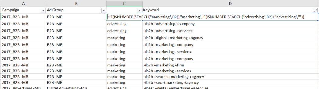
Taking things a step further, let’s say you want to see how keywords containing “marketing” are performing versus keywords containing “advertising.” Nest the same function in the FALSE portion of the previous formula, replacing “marketing” with “advertising.”

PLEASE NOTE: It is best to retype this Excel formula directly into Excel. The code may result in an error when directly pasted.

=IF(ISNUMBER(SEARCH(“marketing”,D2)),”marketing”,IF(ISNUMBER(SEARCH(“advertising”,D2)),”advertising”,””))

Explanation: The formula looks to see if the cell to its right (D2) contains “marketing.” If TRUE, it returns “marketing,” if FALSE it then checks to see if it contains “advertising,” and if that condition is also FALSE it returns a blank cell, or “”.

1. 1. Copy the previous formula and paste it into your notepad.
   2. Remove the opening = sign with a comma.
   3. Replace “marketing” with “advertising.”
   4. Copy the revised formula.
   5. Click into cell C2, delete “”)) after the final comma and paste the revised formula.
   6. Filter the cells  “Z to A” like in the previous example.

You can now add a header to column C and create a pivot table comparing the performance of “marketing” versus “advertising” keywords

Stripping Modified Broad (+) Sign:

Reporting on keyword performance for accounts utilizing the same keywords across different match types represents another common challenge.

It should be simple, right?

You change your date range to “all time” and export all keywords.

However, you quickly realize that all modified broad keywords have a (+) sign in front of each word. You try to remove the (+) sign via a Find and Replace, but you’re left with an added space at the start of each keyword.

Avoid this headache by using the following formula:

PLEASE NOTE: It is best to retype this Excel formula directly into Excel. The code may result in an error when directly pasted.

=IF(ISNUMBER(SEARCH(“+”,$D2)),TRIM(SUBSTITUTE($D2,”+”,””)),$D2)

1. 1. Add a column to the left of keyword column D.
   2. Add a header such as “Stripped Keyword” into cell C1.
   3. Past the above formula into cell C2.
   4. Copy the formula down by clicking the box in the lower right corner.
   5. Create a pivot table and select “Stripped Keyword” as the row.

• • • Add “Match Type” below the “Stripped Keyword” row.
  • Add any data such as impressions, clicks, and conversions to break down performance by match type.

Projecting Performance Through End of Month:

Monitoring your marketing budget is extremely important, as is projecting future spending. If you need accurate projections that can’t wait for your regularly scheduled budget analysis, you’ll want a quick and easy way to get estimates based on the latest performance data.

By using these formulas below, you can ensure that your ad spend will be aligned with your budget come the end of the month.

• • Date Formulas:
    • • Today’s Date: Cell A2
        • =TODAY()
    • • End of Month: Cell B2
        • =EOMONTH(A2,0)
    • Days Left in Month: Cell C2
      • =(B2-A2)+1

• Projection Formula:
  • =“MTD Cost”+(( “Last 7 Days”/7)*Days Left)

Explanation: The “End of Month” and “Days Left in Month” formulas refer to “Today’s Date” to take the last seven days of performance and calculate performance to the end of the month.

The formula takes the last seven days’ performance, divides it by seven for the average daily performance, and multiplies that average by the number of days left. Then, it adds that to “spend to date.”

In this example, we use a formula to project ad spend through the rest of the month. Keep in mind that this formula can be used to project other metrics such as clicks or conversions, too.

1. 1. Pull data from the applicable platform, with the campaign name in column A, the last seven days’ spend in column B, and spend to date for the current month in column C.
      • Do not include the current day’s performance.
   2. Insert three rows above the data table created in the previous step. Our three date calculation formulas will go on line 2, with their headers directly above in line 1.
      • In cell A2 type =TODAY(). Which, as I’m sure you’ve already figured out, returns today’s date.
      • In B2, enter =EOMONTH(A2,0). This formula references today’s date in A2 and returns the last day of the month.
      • In C2, enter =(B2-A2)+1. This subtracts today from the month’s last day and adds one day so to include today. This returns how many days are left in the current month.
      • Type headers in cells A1, A2, and A3 for easy reference.
   3. Type “Projected Spend into the table header row in column D (D4) and enter the following formula below in cell D5:
      =C5+((B5/7)*$C$2) 
      • • The parentheses takes “Last 7 Days” spend in Column B and divides it by seven, which gives you the average spend per day over the past seven days.
      • • The average spend per day is then multiplied by the number of remaining days in cell $C$2, which projects spend for the remainder of the month.
      • • The projected spend is then added to “Spend to Date” in column C.
      • • Copy the cell down to the bottom of your data table. The dollar signs make this cell an absolute formula, allowing you to copy the formula down while keeping the reference to cell C2.
   4. In column D, click into the cell immediately below your table, then click the “AutoSum” button on the top right of the Excel Toolbar and hit “Enter”. This will total the projected monthly spend for all campaigns in the table.

Excel for Marketers — Expand Your Toolkit

While we used PPC examples, data analysis is critical for all advertising and marketing efforts. Our team has developed tools and methods to make us more efficient, and Excel has proven to be indispensable.

Excel for marketers is like a muscle that needs to be flexed every once in a while. If you don’t learn new ways of using Excel, you will be less efficient and miss out on potential opportunities.   

If you’re interested in learning how you can drive better results with digital advertising, learn more about how to receive a free Google AdWords audit.